In my last post I developed a solution to OpenAI Gym’s CartPole environment, based on a classical Q-Learning algorithm. The best score I achieved with it was 120, although the score I uploaded to the leaderboard was 188. While this is certainly not a bad result, I wondered if I could do better using more advanced techniques. Besides that I also wanted to practice the concepts I had recently learned in the Machine Learning 2 course at university. By the way, to all the students among you: I found that one of the best way to learn about new algorithms etc. is to actually try to implement them in code!
Motivation
One major limitation of my classical Q-Learning approach was that the number of possible states had to be reduced from basically infinity (due to the observations’ continuous nature) to, in my case, 1 * 1 * 6 * 12 = 72 discrete states. Considering this extreme simpification, the results were astonishingly good! However, what if we could utilize more of the information, the observations give us? One solution is to combine Q-Learning with a (deep) neural network, which results in a technique called Deep Q-Learning (DQN). Neural networks are inherently efficient when handling very high dimensional problems. That’s why they are doing so well with image-, video- and audio data. Additionally, they can easily handle continuous inputs, whereas with our classical approach we needed the Q-table to be a finite (in this case (4+1)-dimensional) matrix (or tensor). Accordingly, with DQN we don’t need discrete buckets anymore, but are able to directly use the raw observations.
Deep Q-Learning
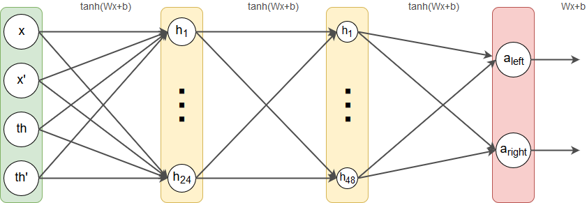
But how does this even work? While I don’t want to explain DQN in detail here, the basic idea is to replace the Q-table by a neural network, which is trained to predict Q-values for a state. The input is a state-vector (or a batch of such) - consisting of four features in this case (which corresponds to four input neurons). The output is a vector of Q-values, one for each possible action - two in our case (corresponding to two output neurons). The training is done using experience replay. Basically, the agent begins to try some random actions and stores its “experiences” into a memory. An experience is a tuple like (old_state, performed_action, received_reward, new_state). At fixed intervals (e.g. after each training episode, but NOT after each step), batches are sampled from memory and used as training data for the network. Consequently, the network (hopefully) improves every episode and predicts more precise Q-values for state-action pairs.
My implementation
My implementation is essentially based on this great blog post by Keon. It uses Keras as a high-level abstraction on top of TensorFlow. However, while I adopted the general structure, I made several tweaks and fixes to massively improve performance.
Tweak #1: More hidden neurons
I slightly modified the network layout by doubling the number of hidden neurons in the second hidden layer. While randomly experimenting with some layouts I found that this one seemed to work better on average. Generally, determining a neural network’s layout is basically trial and error for the most parts. Mainly you want to master the bias-variance tradeoff, but there is no rule on how to choose network structure in order to do so. Mine looks like this now:

Tweak #2: Larger replay memory
In Keon‘s original implementation, the replay memory had a maxmimum size of 2,000. Assuming an average “survival” time of 100 steps, it would only hold experiences from 20 episodes, which is not much. I didn’t see any reason why they shouldn’t be a greater variety in training examples, so I increased the memory size to 100,000.
Tweak #3: Mini-batch training
While originally the network trained from batches of 32 examples in each episode, the way the training was conducted was not efficient in my opinion. Instead of giving TensorFlow a 32 x 4 matrix, it was given a 1 x 4 matrix 32 times, so the actual training procedure effectively used a mini-batch size of 1. Without having technical knowledge on how TensorFlow works, I’m still pretty sure that training the network with one large batch instead of 32 small ones is faster - especially when using a GPU.
Tweak #4: Setting γ = 1
As already mentioned in my last post, I’m of the opinion that it wouldn’t make sense to set the gamma parameter to less than one. Its purpose is to “penalize” the agent if it takes long to reach its goal. However, in CartPole its even our goal to do as many steps as possible.
Tweak #5: Logarithmic ε-decay
Since the adaptive exploration rate from @tuzzer’s solution was very effective in my last implementation, I simply adopted it for this one, too. I didn’t cross-validate whether it’s better or worse than Keon‘s epsilon decay, but at least it doesn’t seem to do bad.

Tweak #6: tanh activation function
I’m really not sure about this point, so please correct me if I’m wrong. The original implementation used the ReLU activation function, which is a linear function that maps the input to itself, but thesholded at zero.

However, since the input features can be negative, ReLU might cause dead neurons, doesn’t it? To overcome that problem, I decided to tanh as an activation function.
Tweak #7: Cross-validate hyperparameters
Eventually, I conducted a grid search (using my script from the last time) to find good values for alpha (learning rate), alpha_decay and epsilon_min (minimum exploration rate). It turned out that alpha=0.01, alpha_decay=0.01 and epsilon_min=0.01 seem to work best among all tested values on average.
Results
After all these optimizations, I ran the algorithm several times and the best score I achieved was actually 24. However, I didn’t record that run, so my best score in the leaderboard in 85, which is better then with my classical Q-Learning approach.
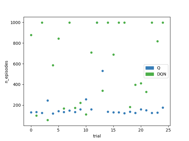
However, I found that although the DQN approach can converge faster, it also seems to be way more unstable at the same time. Performing two consecutive runs of the exact same algorithm and configuration often resulted in one score to be extremely good, while the second one didn’t even solve the environment at all (> 999 episodes). In other words, DQN has a way larger variance, than the table-based approach, as depicted in the chart below, where I performed 25 runs of each algorithm. Additionally, as expected, the neural network is slower. Running DQN 25 times took 744 seconds, while running table-based Q-Learning 25 times only took 24 seconds on my machine’s CPU using four threads on four cores.
>> Code on GitHub (dqn_cartpole.py)

Q: Min 120, Max 999, Mean 197.16, Std: 183.223
DQN: Min 56, Max 999, Mean 600.04, Std: 356.046
Comments